Somewhere along the way, multi cloud stopped being an architecture decision and became a personality trait. It shows up on slide decks the way kale shows up at weddings, nobody is quite sure who asked for it, but removing it now would feel like a confession. Say the words out loud in a meeting and watch the room nod with the solemn confidence of people who have read the headline but not the footnotes.
The pitch is seductive. Spread your workloads across two or three providers and you get freedom, resilience, and a vague aura of technical adulthood. What you actually get, in a surprising number of cases, is a second pager rotation and a networking bill that reads like a ransom note.
This is not an argument that multi cloud is always wrong. It is an argument that it is rarely the default answer to a question nobody bothered to ask. A lot of cloud decisions get made the way people buy treadmills, for the version of themselves they intend to become, not the one currently standing in the room.
What the multi cloud pitch is really selling
Strip away the architecture diagrams, and the multi cloud sales pitch is mostly emotional. It promises escape from vendor lock in, that primal fear of being trapped by a provider who knows it. It offers the warm feeling of resilience, the sense that if one cloud falls over, your business will calmly stroll to the next one. And it projects maturity, the impression that your team has graduated from amateur hour to serious infrastructure people.
These are real desires. The problem is that multi cloud answers them roughly the way buying a second house answers your fear of a leaky roof. Technically, you now have options. You also have two roofs.
Where the trouble starts
The fantasy version of multi cloud assumes a clean layer of abstraction sitting neatly on top of every provider, so your team writes once and runs anywhere. The practical version is that each cloud is its own country, with its own language, customs, and bewildering opinions about what a load balancer should be called.
Total abstraction almost never survives contact with production. Your engineers do not get to learn one platform deeply. They get to learn two platforms simultaneously, plus the seam between them, which is where the genuinely interesting bugs live. The architecture becomes harder to document, harder to operate, and harder to evolve, which is a polite way of saying nobody on the team fully understands all of it anymore, including the person who built it.
The costs nobody put on the slide
Here is where the war story usually turns grim. The expensive part of multi cloud is rarely the compute. It is everything wrapped around it.
You duplicate your observability stack, because the dashboards that work beautifully in one cloud are politely useless in the other. Your IAM and governance model doubles in surface area, since every permission, role, and policy now needs a twin that behaves identically and never quite does. Network egress, cross cloud replication, and data transfer charges accumulate quietly in the background like a subscription you forgot to cancel.
And then there is the human cost, which never appears in the cost calculator. Multi cloud raises the seniority floor of your entire team. The junior engineer who could safely ship in a single, well governed environment now needs to understand two of everything before they can be trusted near production. You do not just pay for more infrastructure. You pay for more expertise to keep that infrastructure from quietly drifting apart.
Security and compliance, now in stereo
Security people have a particular look they get when you mention multi cloud, the expression of someone who has been asked to childproof two houses for the price of one.
Every additional cloud is another attack surface, another set of policies to keep synchronized, and another generous opportunity for a misconfiguration to go unnoticed. Auditing becomes an exercise in translation, because a control that means one thing in the first provider means something subtly different in the second. The realistic end state is not airtight redundancy. It is an uneven security posture, strong where your team has invested attention and quietly soft where they ran out of hours.
Operations and the art of the unsolvable incident
Incidents are where multi cloud presents its invoice. At three in the morning, when something is on fire, you do not want your logs, metrics, and traces scattered across two providers like a crime scene split between jurisdictions.
Correlating an incident across clouds is slow, and slow is expensive when customers are watching. Mean time to detection creeps up. Mean time to resolution creeps up with it. Postmortems acquire an extra paragraph that always begins with some variation of “we lost time understanding which cloud was actually responsible.” To stitch the picture back together, you end up leaning on yet another external platform whose only job is to make your two clouds look like one, which, if you squint, is a strange amount of effort to undo a decision you made on purpose.
Portability you have versus portability you imagine
The intellectual cornerstone of multi cloud is portability, the comforting belief that you could pack up and move providers whenever you liked. In practice, portability tends to be the gym membership of architecture, fully paid for, rarely used, and quietly aspirational.
Most systems end up leaning on provider specific services anyway, because those services are good and saying no to them on principle is a luxury few teams can afford. Kubernetes and containers genuinely help, they smooth the edges, but they do not magically erase the dependency underneath. Real migrations are still slow, still costly, and still the kind of project that gets proposed with enthusiasm and abandoned with relief.
The honest goal is not total independence. It is a reasonable exit, an architecture where leaving would be painful but possible, rather than one where leaving is theoretically free and practically unthinkable. Designing for a sensible escape route beats promising a freedom you will never exercise.
When multi cloud actually earns its keep
None of this means multi cloud is a mistake. It means it is a tool with a narrow, legitimate set of jobs, and it deserves to be used for those rather than worn as a badge.
It earns its place when regulation or data sovereignty leaves you no choice, when the data legally must live in particular places. It makes sense when your organization is large enough that real negotiating leverage over providers translates into serious money. It is justified when the business risk is so high that genuine cross cloud redundancy is worth its considerable price. It is reasonable when a specific service on another cloud offers an advantage you cannot replicate elsewhere. And it works, crucially, only when the organization is mature enough to operate it, with the teams, processes, and discipline already in place rather than hopefully on order.
Notice that every one of these starts with a concrete business reason, not a vibe.
What I would do instead
If you handed me a blank slate and a reasonable budget, I would pick one primary cloud and govern it properly, because a single environment run well beats two environments run anxiously almost every time.
I would design for enough portability to sleep at night, not for the fantasy of frictionless migration. I would automate deployments and infrastructure from day one, before the shortcuts calcify into tradition. I would standardize observability, security, and cost management so the whole thing stays legible to the people who did not build it. And I would revisit the single cloud decision on a schedule, honestly, looking for a real reason to expand rather than a fashionable one.
That last part matters. The goal is not loyalty to one provider. It is refusing to add a second one until something other than anxiety is asking for it.
The question worth asking
Multi cloud can be genuinely useful. It just should not be the reflex, the thing you reach for because the alternative feels insufficiently ambitious. Far too often, what gets sold as strategy is simply complexity wearing a nicer outfit.
Cloud maturity is not measured in the number of providers on your invoice. It is measured by how well you use the one you actually need. The most sophisticated architecture in the room is frequently the one that resisted the urge to be impressive.
So the question is not how many clouds you run. It is whether each one earns its place.
It was 3 AM on a Sunday when the primary database finally gave up. The alerts did not scream about a traffic spike or a rogue deployment. Instead, the culprit was a seemingly innocent Kubernetes CronJob named report-generator-weekly. Thanks to a subtle daylight saving time shift and a misunderstanding of how the kubelet interprets timezones, the cluster decided to spawn twenty-five concurrent instances of a highly unoptimized SQL aggregation query. The database wept, the API went down, and a dozen pagers ruined a perfectly good weekend.
Scheduled jobs can seem deceptively simple until they disrupt production. We tend to treat Kubernetes as a universal solvent for all our operational problems. If it runs containers, it should handle a little task scheduling, right? Sadly, the reality is far more complicated. Behind the scenes, the timezone handling often defaults to the kubelet’s local clock, concurrency policies are treated as polite suggestions under heavy control plane load, and failed jobs accumulate in your cluster like dirty dishes in a shared office sink. Observability is fractured across transient pods, ephemeral events, and missing logs. These “small” details are precisely how a benign script turns into an incident vector.
Resource contention and the illusion of isolation
Your scheduled job does not care about your Service Level Agreements. When you deploy a CronJob into a shared cluster, you are introducing a highly unpredictable workload into the same ring where your latency-sensitive APIs reside. Kubernetes tries its best to balance the scales, but the scheduler is only as good as the resource requests you provide.
Most scheduled jobs are spiky. They sleep for 23 hours, wake up, devour every megabyte of RAM they can reach, and then vanish. If you underprovision the memory requests to save money, the OutOfMemory killer will brutally terminate your job midway through a critical payment reconciliation. If you overprovision to stay safe, you end up paying for idle compute across your worker nodes all day long. We have all seen clusters where a five-minute data cleanup task was given the same IAM permissions and CPU priority as the core stateful application simply because “it is just a cron”. Taints, tolerations, and node affinity help, but they often create a false sense of isolation while increasing scheduling complexity.
Managed schedulers and workflow patterns to the rescue
The smartest way to run a CronJob in Kubernetes is usually to not run it in Kubernetes at all. If you are already building on a major cloud provider, you have access to tools that were specifically designed for this exact headache.
Consider decoupling the “schedule” from the “work”. Services like Cloud Scheduler in GCP, EventBridge in AWS, or Azure Logic Apps are practically bulletproof when it comes to firing a trigger at a specific time. You can wire these services to invoke a Cloud Run service, a Lambda function, or an ECS Fargate task. Yes, there is a minor trade-off regarding vendor lock-in. However, the operational peace of mind you gain by offloading scheduling logic to a managed service usually pays for itself during the first month.
For more complex scenarios where jobs depend on each other, you should look toward delay queues like SQS or Pub/Sub, or dedicated workflow engines like Temporal. When a scheduled task fails halfway through, a pure Kubernetes CronJob will either restart from scratch or die entirely. A proper workflow engine provides built-in backoff logic, idempotent execution tracking, and distributed state management. This pattern beats the traditional cron daemon every time you need reliable retries.
Hardening your jobs and the beauty of boring virtual machines
Of course, there are times when you absolutely must run scheduled jobs inside the cluster. I have also copied-pasted a CronJob YAML file at 2 AM out of sheer necessity (we have all been there). If you find yourself in this situation, you need to establish some defensive boundaries.
Start by enforcing resource quotas per cron namespace to contain the blast radius. Make idempotency checks mandatory in your application code, ensuring that a job running twice by accident does not charge a customer twice. Implement structured logging with clear correlation IDs so you can actually trace failures, and use preStop hooks for graceful shutdowns. The Kubernetes documentation clearly states that a CronJob might run a job zero times or multiple times under certain edge cases, so your code must defend itself against the infrastructure.
Alternatively, we should revive our appreciation for systemd timers on basic Virtual Machines. If you have a low-frequency, highly predictable job that is critical to your infrastructure, a lightweight VM is a fantastic home for it. Systemd timers are exceptionally reliable, the cost is completely transparent, and the blast radius is physically isolated from your stateless microservices. Reserving Kubernetes for your scalable workloads while putting the boring, critical timers on a VM is not a step backward. It is just good engineering.
A plea for architectural humility
Kubernetes is a brilliant piece of software. It is an exceptional orchestrator for stateless, auto-scaling microservices. However, it is not a magical alarm clock, and treating it as a universal cron daemon is a recipe for operational misery.
Architectural humility means picking the right tool for the job, rather than the trendiest one. The next time someone proposes adding a heavy, stateful CronJob to the production cluster, take a moment to ask the hard questions about resource profiles, failure tolerance, and observability. Sometimes, the most advanced cloud architecture decision you can make is to let a dedicated scheduling service handle the calendar, leaving your cluster free to do what it does best.
Let us consider the cranium of the modern Cloud Architect. It is a finite biological container, roughly the size of a cantaloupe, filled with a squishy mass of fat and water. Yet, the tech industry operates under the hallucination that this cantaloupe can effortlessly absorb the entire AWS service catalog updates before your morning coffee. Trying to ingest the sheer volume of new DevOps tooling is a lot like watching a python try to swallow a double-door refrigerator. It is structurally impossible, deeply uncomfortable to witness, and usually ends with someone needing medical attention. We are practically obligated to evolve constantly, but our neurological hard drives have strict, unyielding limits.
The biological absurdity of keeping up with the CNCF landscape
The concept of “continuous improvement” in IT often feels less like an inspirational corporate poster and more like a slightly sadistic evolutionary mandate. You finally understand the esoteric routing logic of your Kubernetes networking setup. Your heart rate settles. You feel peace. Then, a cheerful newsletter arrives to inform you that your setup is obsolete and someone has thrown a brand new service mesh at your head.
The exhaustion you feel is not a character flaw. It is a standard biological response to an ecosystem that mutates faster than a flu virus in a crowded airport. Our brains were optimized for remembering which berries are poisonous, not for tracking the depreciation schedule of Helm charts.
Stop eating the trendy vegetables you hate
Then there is the fear of missing out, or FOMO, which drives otherwise rational engineers to do deeply irrational things. Let us be brutally honest here. If you absolutely despise Javascript or feel a physical wave of nausea when looking at a shiny new frontend framework, do not force yourself to learn them just because they are trending on Hacker News.
Trying to master disciplines outside your actual interests is like forcing a housecat to take up scuba diving. The cat will hate it, it will do a terrible job, and everyone involved will end up bleeding. Protect your cognitive load with ruthless aggression. As a DevOps professional, you have permission to focus solely on the infrastructure pipelines and Linux kernel quirks that actually bring you joy. Leave the trendy stuff to the people who actually like it.
Enter the hyperactive, infinitely patient robot intern
This brings us to the survival strategy. Artificial intelligence is often pitched as an omniscient overlord coming for our jobs. Right now, however, it is much more useful to view it as a hyperactive, infinitely patient intern. These LLMs exist to do the dirty work our cantaloupe brains reject.
They can read the soul-crushing, poorly translated documentation you desperately want to avoid. You can feed a brutal 50-page technical manual on IAM policies into an AI tool and instruct it to spit out a concise summary directly in your terminal. Or better yet, tell it to explain the concepts to you like you are a tired sysadmin who just wants to go home and play with their Mac. It saves hours of mental decay.
Curating your own survival kit
The trick is learning how to interrogate the AI properly. You do not just ask it “what is new in Terraform.” You demand it to extract the protein from the learning material and throw away the useless fat. You can ask it to summarize release notes, generate highly specific flashcards, or even act as a mock interviewer to test your knowledge on specific CI/CD pipelines before a migration. You are outsourcing the most painful parts of the learning curve to a machine that cannot feel pain or boredom.
The fine art of ignoring things
Ultimately, surviving this industry requires a liberating realization. You simply cannot know everything, and attempting to do so is a biological folly. To truly master the fine art of ignoring things, you need to implement a few practical, slightly ruthless habits.
First, practice strategic amnesia. Stop trying to memorize syntax. If an AI can generate the boilerplate YAML for a Kubernetes deployment in three seconds, your brain should actively refuse to store that information. Treat syntax like a disposable coffee cup; use it once and throw it away.
Second, stop hoarding documentation and start hoarding prompts. Your personal knowledge base should not be a graveyard of unread PDFs. It should be a collection of highly tuned, tested instructions that you can feed into an LLM to get exactly what you need, when you need it. Think of them as spells to summon your robot intern.
Third, politely decline the buffet. When a vendor announces a revolutionary new tool that solves a problem you do not actually have, just nod, smile, and walk away. Your cognitive load is precious cargo. Do not fill the cargo bay with garbage.
The ultimate architectural achievement is not memorizing every obscure command line flag. It is building a well structured mind that understands the core principles and knows exactly how to extract the rest of the answers from an AI assistant. Let the machines hold the heavy encyclopedias. We need our brain space for the truly important mysteries, like figuring out why the production database just mysteriously vanished.
The internet has many glamorous job titles. Cloud architect. Platform engineer. Security specialist. Site reliability engineer, which sounds like someone hired to keep civilization from sliding gently into a ditch.
DNS has none of that glamour.
DNS is the receptionist sitting at the front desk of the internet, quietly answering the same question billions of times a day.
Where is this thing?
You type a name like “www.example.com”. Your browser nods with confidence, like a waiter who has written nothing down, and somehow a website appears. Behind that small miracle is DNS, the Domain Name System, a distributed naming system that turns human-friendly names into machine-friendly addresses.
Humans like names. Computers prefer numbers. This is one of the many reasons computers are not invited to dinner parties.
Without DNS, using the internet would feel like trying to visit every shop in town by memorizing its tax identification number. Possible, perhaps, but only for people who alphabetize their spice rack and have strong opinions about subnet masks.
DNS lets us type names instead of IP addresses. It maps domain names to the information needed to reach services, send email, verify ownership, issue certificates, and keep many small pieces of infrastructure from wandering into traffic.
It is boring in the way plumbing is boring. Nobody praises it when it works. Everybody becomes a philosopher when it breaks.
Why DNS exists
When you visit a website, your browser needs to know where that website lives. The name “google.com” is useful to you, but it is not directly useful to the machines moving packets across networks.
Those machines need IP addresses.
An IPv4 address looks like this.
142.250.184.206
An IPv6 address looks like this.
2a00:1450:4003:80f::200e
IPv6 addresses are what happens when a numbering system grows up, gets a mortgage, and decides readability is no longer its problem.
The basic job of DNS is to answer questions such as this.
What IP address should I use for www.example.com?
And then DNS replies with an answer such as this.
www.example.com -> 93.184.216.34
That is the simple version. It is true enough to be useful, but not complete enough to explain why DNS can ruin your afternoon while wearing the innocent expression of a houseplant.
The more accurate version is that DNS is a distributed, hierarchical, cached database. No single server knows everything. Instead, different parts of the DNS system know different parts of the answer, and resolvers know how to ask the right questions in the right order.
The internet’s receptionist does not keep every phone number in one drawer. That would be madness, and also suspiciously like a spreadsheet someone named Martin promised to maintain in 2017.
What happens when you type a domain name
When you type a website address into your browser, your machine does not immediately interrogate the entire internet. It starts closer to home, because even computers understand that walking across the office to ask a question is embarrassing if the answer was already on your desk.
A simplified DNS lookup usually works like this.
The browser checks whether it already knows the answer.
The operating system checks its own DNS cache.
The request may go to your router, corporate DNS, ISP resolver, or a public resolver such as Google DNS or Cloudflare DNS.
If the resolver does not already have the answer cached, it starts asking the DNS hierarchy.
It asks the root DNS servers where to find the servers for the top-level domain, such as .com.
It asks the .com servers where to find the authoritative nameservers for the domain.
It asks the authoritative nameserver for the actual record.
The IP address comes back.
Your browser connects to the server.
The website loads, assuming the rest of the internet has decided to behave.
This process often happens in milliseconds. It is quick enough to look like magic and structured enough to be bureaucracy.
That distinction matters.
Magic cannot be debugged. Bureaucracy can, provided you know which desk lost the form.
Recursive resolvers and authoritative nameservers
Two DNS roles are worth understanding early, because they explain a lot of real-world behavior.
The first is the recursive resolver.
This is the DNS server your device asks for help. It does the legwork. Your laptop says, “Where is www.example.com?” and the recursive resolver goes off to find the answer. It may already know the answer from cache, or it may need to ask other DNS servers.
The recursive resolver is the intern sent across the building with a clipboard and mild panic.
The second is the authoritative nameserver.
This is the DNS server that holds the official answer for a domain or zone. If a domain uses a particular DNS provider, such as Route 53, Cloud DNS, Cloudflare, or another provider, that provider’s authoritative nameservers are responsible for answering questions about the records configured there.
The authoritative nameserver is the person with the spreadsheet, the badge, and the unsettling confidence.
This difference matters because your laptop usually does not ask the authoritative nameserver directly. It asks a resolver. The resolver may answer from cache. That is why one person sees the new DNS record and another person, in the same meeting, sees the old one and begins quietly questioning reality.
DNS records are tiny instructions with large consequences
A DNS record is a piece of information stored in a DNS zone. It tells DNS what should happen when someone asks about a name.
A domain without DNS records is like an office building with no signs, no mailbox, no receptionist, and one confused courier holding your production traffic.
DNS records decide things like these.
Which IP address serves a website
Which hostname acts as an alias
Which servers receive email
Which systems are allowed to send email for a domain
Which certificate authorities may issue TLS certificates
Which nameservers are responsible for the domain
Which services exist under specific names
If DNS records are wrong, the result is rarely poetic. Websites stop loading. Email disappears into procedural fog. Certificates fail. Monitoring dashboards develop a sudden interest in the color red.
DNS records look small, but they carry adult responsibility.
A and AAAA records
The A record is the most basic DNS record. It maps a name to an IPv4 address.
example.com -> 192.0.2.10
This record says, with refreshing directness, “This name lives at this IPv4 address.”
The AAAA record does the same job for IPv6.
example.com -> 2001:db8:1234::10
A and AAAA records are common when you control the target IP address. For example, you may point a domain to a virtual machine, a static endpoint, or a load balancer with stable addresses.
In modern cloud environments, however, you often do not want to point directly to a single server. You may want to point to a load balancer, a CDN, or a managed service whose underlying IPs can change. That is where aliases and provider-specific features become important.
DNS is simple until cloud infrastructure arrives wearing three badges and carrying a YAML file.
CNAME records
A CNAME record creates an alias from one DNS name to another DNS name.
blog.example.com -> example-blog.provider.com
This does not work like an HTTP redirect. That distinction is important.
A browser redirect says, “Go to a different URL.”
A CNAME says, “This DNS name is really another DNS name. Ask about that one instead.”
It is not a forwarding service. It is an alias.
CNAME records are especially useful for subdomains. For example, you may point docs.example.com to a documentation platform, or shop.example.com to an e-commerce provider.
One important rule is that a CNAME normally cannot coexist with other records at the same name. If blog.example.com is a CNAME, it should not also have MX or TXT records at that exact same name. DNS dislikes identity crises.
Also, the root domain, often called the zone apex, such as example.com, usually cannot be a standard CNAME because it must have records like NS and SOA. Many DNS providers solve this with records called ALIAS or ANAME, or with provider-specific alias features.
For example, AWS Route 53 has Alias records, which are not a normal DNS record type but are extremely useful when pointing a root domain to an AWS load balancer, CloudFront distribution, or another AWS target.
The practical lesson is simple. Use CNAMEs for aliases when allowed. Use your DNS provider’s supported alias mechanism when dealing with root domains and cloud-managed targets.
This is DNS saying, “There are rules, but we have invented paperwork to survive them.”
MX records
MX records tell the world where email for a domain should be delivered.
example.com -> mail.example.com
In real DNS, MX records also have priorities. Lower numbers are preferred.
This means mail servers should try mail1.example.com first, and use mail2.example.com as a fallback.
MX records matter because email is not delivered to your website. It is delivered to mail servers responsible for your domain. This is why a website can work perfectly while email is broken, and everyone involved can be technically correct while still being deeply unhappy.
Email uses DNS heavily. MX records route the mail. TXT records help prove which systems are allowed to send it. PTR records may help receiving systems trust the sending server. Email security is basically DNS wearing a trench coat full of paperwork.
TXT records
TXT records store text. That sounds harmless, like a sticky note, until you realize that half the modern internet uses sticky notes to prove ownership, configure email security, and convince platforms that you are not a spam goblin.
TXT records are also used for domain verification. Google, Microsoft, GitHub, certificate providers, and many SaaS platforms may ask you to create a TXT record to prove that you control a domain.
The humble TXT record is DNS with a clipboard and a suspicious number of compliance responsibilities.
NS and SOA records
NS records define which nameservers are authoritative for a domain or zone.
Without correct NS records, resolvers may not know where to ask for official answers. That is a problem, because DNS without authority is just gossip with port 53.
SOA stands for Start of Authority. Every DNS zone has an SOA record. It contains administrative information about the zone, including the primary nameserver, contact details, serial number, and timing values used by secondary nameservers.
You usually do not edit SOA records during basic DNS work, but they exist behind the scenes. They are the domain’s administrative birth certificate, stored in a filing cabinet that occasionally matters a lot.
PTR records and reverse DNS
Most DNS lookups turn names into IP addresses. A PTR record does the reverse. It maps an IP address back to a name.
192.0.2.10 -> server.example.com
This is called reverse DNS.
Reverse DNS is often used in email systems, logging, security investigations, and operational troubleshooting. If a mail server sends email from an IP address, receiving systems may check whether reverse DNS makes sense. If it does not, the email may look suspicious.
PTR records are usually managed by whoever controls the IP address range, often a cloud provider, hosting provider, or network team. This is why you may control example.com but still need to configure reverse DNS somewhere else.
DNS enjoys reminding us that ownership is a layered concept, like lasagna or enterprise access management.
SRV and CAA records
SRV records describe where specific services are available. They are often used by systems such as VoIP, chat, directory services, or service discovery mechanisms.
An SRV record can include the service name, protocol, priority, weight, port, and target host.
_service._tcp.example.com -> target.example.com on port 443
Many people can use DNS for years without touching SRV records. Then one day a system requires them, and SRV appears like a cousin nobody mentioned during onboarding.
CAA records control which certificate authorities are allowed to issue TLS certificates for your domain.
example.com CAA 0 issue "letsencrypt.org"
This tells certificate authorities that Let’s Encrypt is allowed to issue certificates for the domain. Other certificate authorities should not.
CAA is a useful security control. It is not a magic shield, but it reduces the risk of unauthorized certificate issuance. Think of it as a small velvet rope in front of your TLS certificates. Not glamorous, but better than letting the entire street into the building.
TTL and the myth of DNS propagation
TTL means Time To Live. It tells DNS resolvers how long they may cache a DNS answer.
If a record has a TTL of 3600 seconds, a resolver can cache that answer for one hour.
This is where many DNS misunderstandings are born, raised, and eventually promoted into incident reports.
People often say, “DNS propagation takes time.” The phrase is common, but it can be misleading. DNS changes are not usually pushed across the internet like flyers under apartment doors. Most of the time, you are waiting for cached answers to expire.
If a resolver cached the old IP address five minutes before you changed the record, and the TTL was one hour, that resolver may continue returning the old answer until the cache expires.
A low TTL can make changes appear faster, but it can also increase DNS query volume. A high TTL reduces query volume, but it makes mistakes more persistent.
This is the technical equivalent of writing something in permanent marker because it felt efficient at the time.
Before planned DNS changes, teams often lower TTL values in advance. For example, if a record currently has a TTL of 86400 seconds, which is 24 hours, you might reduce it to 300 seconds a day before migration. Then, when you switch the record, cached answers expire much faster.
After the migration is stable, you may increase the TTL again.
This is not exciting work. It is careful work. DNS rewards careful people by giving them fewer reasons to age visibly during production changes.
Common ways DNS breaks things
DNS failures are rarely introduced with dramatic music. They usually arrive disguised as simple user complaints.
“The website is down.”
“Email is not arriving.”
“It works from my machine.”
“The old environment is still receiving traffic.”
These are not always DNS problems, but DNS should be part of the investigation.
Common issues include these.
An A record points to the wrong IP address.
A CNAME points to the wrong target.
A record was changed, but resolvers still have the old answer cached.
Nameservers at the registrar do not match the DNS provider where records were edited.
MX records are missing or misconfigured.
TXT records for SPF, DKIM, or DMARC are incomplete.
A certificate authority cannot issue a certificate because CAA records block it.
Internal and external DNS return different answers, and nobody documented the difference because optimism is cheaper than documentation.
A particularly common mistake is editing DNS records in the wrong place. The domain may be registered with one company, but the authoritative DNS may be hosted somewhere else. Changing records at the registrar will do nothing if the authoritative nameservers point to another DNS provider.
This is how people end up pressing Save repeatedly in a web console while DNS stares politely from another building.
DNS in cloud and DevOps
For cloud, DevOps, and platform engineering work, DNS is not optional background noise. It is where architecture becomes reachable.
A Kubernetes Ingress may expose an application through a cloud load balancer. DNS must point the application hostname to that load balancer.
A CDN such as CloudFront or Cloud CDN may sit in front of an application. DNS must point users toward the CDN, not directly to the origin.
A managed database, API gateway, object storage website, or SaaS platform may require CNAMEs, TXT verification records, private endpoints, or provider-specific aliases.
In AWS, Route 53 Alias records are commonly used to point domains to AWS resources such as Application Load Balancers or CloudFront distributions.
In GCP, Cloud DNS can host public or private zones, and DNS can be part of the design for internal services, private connectivity, and hybrid architectures.
In Kubernetes, internal DNS also matters. Services get names inside the cluster. Pods can call other services using names such as this.
my-service.my-namespace.svc.cluster.local
That internal DNS is different from public DNS, but the idea is related. Names hide moving parts. Services can change IP addresses. Pods can die and be replaced. DNS gives workloads a stable name to use while the infrastructure performs its little disappearing act.
Cloud architecture is full of things that move, scale, fail, restart, and get replaced. DNS is one of the systems that lets users pretend this is all very stable.
Bless DNS for its emotional labor.
Useful DNS troubleshooting commands
You do not need many tools to begin troubleshooting DNS. A few commands can reveal a lot.
Use dig to query DNS records.
dig example.com A
Query a specific resolver.
dig @8.8.8.8 example.com A
Check MX records.
dig example.com MX
Check TXT records.
dig example.com TXT
Trace the delegation path.
dig example.com +trace
Use nslookup if it is what you have available.
nslookup example.com
Use host for quick lookups.
host example.com
For operational troubleshooting, compare answers from different resolvers. Your corporate DNS, Google DNS, Cloudflare DNS, and the authoritative nameserver may not all return the same answer at the same time, especially after a recent change.
That does not always mean DNS is broken. Sometimes it means DNS is being DNS, which is not comforting, but it is accurate.
When the receptionist leaves the desk
DNS is one of those technologies that feels simple until you need to explain why production traffic is still going to the old load balancer, why email authentication broke after a migration, or why half the office sees the new website, and the other half appears trapped in yesterday.
At its heart, DNS turns names into answers.
But in real systems, those answers are cached, delegated, aliased, verified, prioritized, and sometimes misfiled in a place nobody checked because the meeting was already running long.
If you work with Linux, cloud, Kubernetes, DevOps, security, networking, or web platforms, DNS is not optional. It is one of the quiet foundations underneath everything else.
It does not look dramatic on architecture diagrams. It does not usually get its own epic in Jira. It does not wear a cape. It sits at the desk, answers questions, points traffic in the right direction, and receives blame with the exhausted dignity of someone who has been doing everyone else’s routing work for decades.
DNS is the internet’s most underpaid receptionist.
And when that receptionist goes missing, nobody gets into the building.
If your pants feel a little tight after a large Thanksgiving meal, the logical solution is to discreetly unbutton them. You do not typically hire a hitman to assassinate yourself, clone your DNA in a vat, and grow a slightly wider version of yourself just to digest dessert. Yet, for nearly a decade, this is exactly how Kubernetes handled resource management.
When an application slowly consumed all its allocated memory, the standard orchestration response was absolute, violent destruction. We did not give the application more memory. We shot it in the head, deleted its entire existence, and span up a brand new replica with a slightly larger plate. Connections dropped. Warm caches evaporated. State was lost in the digital wind.
Thankfully, the era of the Kubernetes firing squad is drawing to a close. In-place pod resizing has officially graduated to stable General Availability in Kubernetes v1.35, and it changes the fundamental physics of how we manage workloads. We can finally stop burning down the house just to buy a bigger sofa.
Let us explore how this works, why it is practically miraculous, and how to use it without accidentally angering the Linux kernel.
The historical absurdity of pod resource management
Before in-place resizing, if you wanted to change the CPU or memory allocated to a running pod, the workflow was brutally simplistic. You updated your Deployment specification with the new resource requests and limits. The Kubernetes control plane saw the discrepancy between the desired state and the current state. The control plane then instructed the Kubelet to terminate the old pod and create a new one.
Think of taking your car to the mechanic because you need thicker tires. Instead of swapping the tires, the mechanic puts your car into an industrial crusher, hands you an identical car with thicker tires, and tells you to reprogram your radio stations. Sure, the rolling update strategy ensured you had a backup car to drive while the primary one was being crushed, but the specific pod doing the heavy lifting was gone.
For stateless microservices written in Go, this was barely an inconvenience. For a massive Java Virtual Machine holding gigabytes of cached data, or a machine learning inference service handling a traffic spike, a restart was a traumatic event. It meant minutes of downtime, CPU spikes during startup, and a slew of unhappy alerts.
Enter the era of in-place resizing
The magic of Kubernetes v1.35 is that the “resources.requests” and “resources.limits” fields within a pod specification are no longer immutable. You can edit them on the fly.
Under the hood, Kubernetes is finally taking full advantage of Linux control groups (cgroups). A container is basically just a regular Linux process trapped in a highly restrictive administrative box. The kernel has always had the ability to move the walls of this box without killing the process inside. If a container needs more memory, the kernel simply adjusts the cgroup memory limit. It is like a landlord quietly sliding a partition wall outward while you are still sleeping in your bed.
Here is a sanitized example of how you might update a running pod. Notice how we are just applying a patch to an existing, actively running resource.
# We patch the running pod to increase memory limits
# No restarts, no dropped connections, just instant gratification
kubectl patch pod bloated-legacy-api-7b89f5c -p '{"spec":{"containers":[{"name":"main-app","resources":{"limits":{"memory":"4Gi"}}}]}}'
It feels almost illegal the first time you do it. The pod keeps running, the uptime counter keeps ticking, but suddenly the application has breathing room.
The bureaucratic lifecycle of asking for more RAM
Of course, you cannot just demand more resources and expect the universe to instantly comply. The physical node hosting your pod must actually have the spare CPU or memory available. To manage this negotiation, Kubernetes introduces a new field in the pod status called resize.
This field tracks the bureaucratic process of your resource request. It is very much like dealing with the Department of Motor Vehicles, but measured in milliseconds. The statuses are surprisingly descriptive.
First, there is Proposed. This means your request for more resources has been acknowledged. The paperwork is on the desk, but nobody has stamped it yet.
Second, we have “InProgress”. The Kubelet has accepted the request and is currently asking the container runtime (like containerd or CRI-O) to adjust the cgroup limits. The walls are physically moving.
Third, you might see Deferred. This is the orchestrator politely telling you that the node is currently full. Your pod is on a waitlist. As soon as another pod terminates or frees up space, your resize request will be processed. You do not get an error, but you also do not get your RAM. You just wait.
Finally, there is Infeasible. This is Kubernetes looking at you with deep, profound disappointment. You probably asked for 64 Gigabytes of memory on a tiny virtual machine that only has 8 Gigabytes total. The API server essentially stamps your form with a big red “DENIED” and moves on with its life.
Negotiating with stubborn runtimes using resize policies
Not all applications are smart enough to realize they have been gifted more resources. Node.js or Go applications will happily consume newly available CPU cycles without being told. Java applications, on the other hand, are like stubborn mules. If you start a JVM with a maximum heap size of 2 Gigabytes, giving the container 4 Gigabytes of memory will accomplish absolutely nothing. The JVM will stubbornly refuse to look at the new memory until you reboot it.
To handle these varying levels of application intelligence, Kubernetes gives us the resizePolicy array. This allows you to define exactly how the Kubelet should handle changes for each specific resource type.
In this configuration, we are telling Kubernetes a very specific set of rules. If we patch the CPU limits, the Kubelet will adjust the cgroups and leave the container alone (RestartNotRequired). The application will just run faster. However, if we patch the memory limits, the Kubelet knows it must restart the container (RestartContainer) so the application can read the new environment variables and adjust its internal memory management.
The vertical pod autoscaler is your marital therapist
Manually patching pods in the middle of the night is still a terrible way to manage infrastructure. The true power of in-place resizing is unlocked when you pair it with the Vertical Pod Autoscaler.
Historically, the VPA was a bit of a brute. It would watch your pods, realize they needed more memory, and then mercilessly murder them to apply the new sizes. It was effective, but highly destructive.
Now, the VPA features a magical mode called InPlaceOrRecreate. Think of this mode as a highly skilled couples therapist. It sits quietly in the background, observing the relationship between your application and its memory usage. When the application needs more space to grow, the VPA simply slides the walls outward without causing a scene. It only resorts to the nuclear option of recreating the pod if an in-place resize is technically impossible.
apiVersion: autoscaling.k8s.io/v1
kind: VerticalPodAutoscaler
metadata:
  name: smooth-scaling-vpa
spec:
  targetRef:
    apiVersion: apps/v1
    kind: Deployment
    name: frontend-service
  updatePolicy:
    # The magic word that prevents the firing squad
    updateMode: "InPlaceOrRecreate"
With this single setting, your stateful workloads, long-running batch jobs, and memory-hungry APIs can seamlessly adapt to traffic spikes without ever dropping a user request.
The fine print and the rottweiler problem
As with all things in distributed systems, there are rules. You cannot cheat the laws of physics. If a node is completely exhausted of resources, your in-place resize will sit in the Deferred state forever. You still need the Cluster Autoscaler to add fresh physical nodes to your cluster. In-place resizing is a tool for distributing existing wealth, not for printing new money.
Furthermore, we must talk about the danger of scaling down. Increasing memory is a joyous occasion. Reducing memory limits on a running container is like trying to take a juicy steak out of the mouth of a hungry Rottweiler.
The Linux kernel takes memory limits very seriously. If your application is currently using 3 Gigabytes of memory, and you smugly patch the pod to limit it to 2 Gigabytes, the kernel does not politely ask the application to clean up its garbage. The Out Of Memory killer wakes up, grabs an axe, and immediately slaughters your application.
Always scale down memory with extreme caution. It is almost always safer to wait for a natural deployment cycle to reduce memory requests than to try to forcefully shrink a running process.
In the end, in-place pod resizing is not just a neat party trick. It is a fundamental maturation of Kubernetes as an operating system for the cloud. We are no longer treating our workloads like disposable cattle to be slaughtered at the first sign of trouble. We are treating them like slightly demanding house pets. Just give them the bigger bowl of food and let them sleep.
Not long ago, a partner I work with told me about a company that decided it had finally had enough of AWS.
The monthly bill had become the sort of document people opened with the facial expression usually reserved for dental estimates. Consultants were invited in. Spreadsheets were produced. Serious people said serious things about control, efficiency, and the wisdom of getting off the cloud treadmill.
The conclusion sounded almost virtuous. Leave AWS, move the workloads to a colocation facility, buy the hardware, and stop renting what could surely be owned more cheaply.
It was neat. It was rational. It was, for a while, deeply satisfying.
And then reality arrived, carrying invoices.
The company spent a substantial sum getting out of AWS. Servers were bought. Contracts were signed. Staff had to be hired to manage all the things cloud providers manage quietly in the background while everyone else gets on with their jobs. Not long after, the economics began to fray. Reversing course costs even more than leaving in the first place.
That is the part worth paying attention to.
Not because it makes for a dramatic story, though it does. Not because it is especially rare, but because it is not. It matters because it exposes one of the oldest tricks in infrastructure decision-making. Companies compare a visible bill with an invisible burden, decide the bill is the scandal, and only later discover that the burden was doing quite a lot of useful work.
The spreadsheet seduction
On paper, the move away from AWS looked wonderfully sensible.
The cloud bill was obvious, monthly, and impolite enough to keep turning up. On-premises looked calmer. Hardware could be amortized. Rack space, power, and bandwidth could be priced. With a bit of care, the whole thing could be made to resemble prudence.
This is where many repatriation plans become dangerously persuasive. The cloud is cast as an extravagant landlord. On-premises is presented as the mature decision to stop renting and finally buy the house.
Unfortunately, a data center is not a house. It is closer to owning a very large hotel whose plumbing, wiring, keys, security, fire precautions, laundry, and unexpected midnight incidents are all your responsibility, except the guests are servers and none of them leave a tip.
The spreadsheet had done a decent job of pricing the obvious things. Hardware. Colocation space. Power. Connectivity.
What was priced badly were all the dull, expensive capabilities that public cloud tends to bundle into the bill. Managed failover. Backup automation. Key rotation. Elastic capacity. Security controls. Compliance support. Monitoring that does not depend on a specific engineer being awake, available, and emotionally prepared.
What looked like cloud excess turned out to include a great deal of cloud competence.
That distinction matters.
A large cloud bill is easy to resent because it is visible. Operational competence is harder to resent because it tends to be hidden in the walls.
What the cloud had been doing all along
One of the costliest mistakes in infrastructure is confusing convenience with fluff.
A managed database can look expensive right up to the moment you have to build and test failover yourself, define recovery objectives, handle maintenance windows, rotate credentials, validate backups, and explain to auditors why one awkward part of the process still depends on a human remembering to do something after lunch.
A content delivery network may seem like a luxury until you try to reproduce low-latency delivery, edge caching, certificate handling, resilience, and attack mitigation with a mixture of hardware, internal effort, procurement delays, and hope.
The company, in this case, had not really been paying AWS only for compute and storage. It had been paying AWS to absorb a long list of repetitive operational chores, specialized platform decisions, and uncomfortable edge cases.
Once those chores came back in-house, they did not return politely.
Redundancy stopped being a feature and became a budget line, followed by an implementation plan, followed by a maintenance burden. Security controls that had once been inherited now had to be selected, deployed, documented, checked, and defended. Compliance work that had once been partly automated became a steady stream of evidence gathering, procedural discipline, and administrative repetition.
Cloud bills can look high. So can plumbing. You only discover its emotional value when it stops working.
The talent tax
The easiest part of moving on premises is buying equipment.
The harder part is finding enough people who know how to run the surrounding world properly.
Cloud expertise is now common enough that many companies can hire engineers comfortable with infrastructure as code, IAM, managed services, container platforms, observability, autoscaling, and cost controls. Strong cloud engineers are not cheap, but they are at least visible in the market.
Deep on-premises expertise is another matter. People who are strong in storage, backup infrastructure, virtualization, physical networking, hardware lifecycle, and operational recovery still exist, but they are not standing about in large numbers waiting to be discovered. They are experienced, expensive, and often well aware of their market value.
There is also a cultural issue that rarely appears in repatriation slide decks. A great many engineers would rather write Terraform than troubleshoot a hardware issue under unflattering lighting at two in the morning. This is not a moral failure. It is simple market gravity. The industry has spent years abstracting away routine infrastructure pain because abstraction is usually a better use of skilled human attention.
The partner who told me this story was particularly clear on this point. The staffing line looked manageable in planning. In practice, it turned into one of the most stubborn and underestimated parts of the whole effort.
Cloud is not cheap because expertise is cheap. Cloud is often cheaper because rebuilding enough expertise inside one company is very expensive.
Why does utilization lie so beautifully
Projected utilization is one of those numbers that becomes more charming the less time it spends near reality.
Many repatriation models assume that servers will be well used, capacity will be planned sensibly, and waste will be modest. It sounds disciplined. Responsible, even.
Real workloads behave less like equations and more like kitchens during a family gathering. There are quiet periods, sudden rushes, abandoned experiments, quarter-end panics, new projects that arrive with urgency and no warning, and services no one remembers until they break.
Elasticity is not a decorative feature added by cloud providers to justify themselves. It is one of the main ways organizations avoid buying for peak demand and then spending the rest of the year paying for machinery to sit about waiting.
Without elasticity, you provision for the busiest day and fund the silence in between.
Silence, in infrastructure, is expensive.
A half-used on-premises platform still consumes power, occupies space, demands maintenance, requires patching, and waits patiently for a workload spike that visits only now and then. Spare capacity has excellent manners. It makes no fuss. It simply eats money quietly and on schedule.
This was one of the turning points in the story I heard. Forecast utilization turned out to be far more flattering than actual utilization. Once that happened, the economics began to sag under their own good intentions.
The cost of becoming slower
Traditional total-cost comparisons handle direct spending reasonably well. They are much worse at pricing lost momentum.
When a company runs on a large cloud platform, it does not merely rent infrastructure. It also gains access to a constant flow of improvements and options. Better analytics tools. New security integrations. Managed AI services. Identity features. Database capabilities. Deployment patterns. Networking enhancements. Observability tooling.
No single addition changes everything overnight. The effect is cumulative. It is a thousand small conveniences arriving over time and sparing teams from having to rebuild ordinary civilization every quarter.
An on-premises platform can be stable and well run. For the right workloads, that may be perfectly acceptable. But it does not evolve at the pace of a hyperscaler. Upgrades become projects. New capabilities require procurement, testing, staffing, and patience. The platform becomes more careful and, usually, slower.
That slower pace does not always show up neatly in a spreadsheet, but engineers feel it almost immediately.
While competitors are experimenting with new managed services or shipping new capabilities faster, the repatriated organization may be spending its time improving backup procedures, standardizing tools, negotiating maintenance arrangements, or replacing hardware that has chosen an inconvenient moment to become philosophical.
There is nothing glamorous about that. There is also nothing free about it.
Who should actually consider on-premises
None of this means on-premises is foolish.
That would be a lazy conclusion, and lazy conclusions are where expensive architecture plans begin.
For some organizations, on-premises remains entirely reasonable. It makes sense for highly predictable workloads with very little variability. It can make sense in tightly regulated environments where legal, sovereignty, or operational constraints sharply limit the use of public cloud. And at a very large scale, some organizations genuinely can justify building substantial parts of their own platform.
But most companies tempted by repatriation are not in that category.
They are not hyperscalers. They are not all running flat, perfectly predictable workloads. They are not all boxed in by constraints that make public cloud impossible. More often, they are reacting to a painful cloud bill caused by weak cost governance, poor workload fit, loose architecture discipline, or a lack of serious FinOps.
That is a very different problem.
Leaving AWS because you are using AWS badly is a bit like selling your refrigerator because the groceries keep going off while the door is open. The appliance may not be the heart of the matter.
The middle ground companies skip past
One of the stranger features of cloud debates is how quickly they become binary.
Either remain in public cloud forever, or march solemnly back to racks and cages as if returning to a lost ancestral craft.
There is, of course, a middle ground.
Some workloads do benefit from local placement because of latency, residency, plant integration, or operational constraints. But needing hardware closer to the ground does not automatically mean rebuilding the entire service model from scratch. The more useful question is often not whether the hardware should be local, but whether the control plane, automation model, and day-to-day operations should still feel cloud-like.
That is a much more practical conversation.
A company may need some infrastructure nearby while still gaining enormous value from managed identity, familiar APIs, consistent automation, and operational patterns learned in the cloud. This tends to sound less heroic than a full repatriation story, but heroism is not a particularly reliable basis for infrastructure strategy.
The partner who described this case said as much. If they had explored the middle road earlier, they might have kept the local advantages they wanted without assuming quite so much of the surrounding operational burden.
What a real repatriation audit should include
Any company seriously considering a move off AWS should pause long enough to perform an audit that is a little less enchanted by ownership.
Start with the full cloud picture, not just the line items everyone enjoys complaining about. Include engineering effort, compliance automation, security services, platform speed, operational overhead, and the cost of scaling quickly when demand changes.
Then build the on-premises model with uncommon honesty. Price round-the-clock operations. Price redundancy properly. Price backup and recovery as if they matter, because they do. Price refresh cycles, maintenance contracts, spare capacity, patching, testing, physical security, audit evidence, and the awkward certainty that hardware fails when it is least convenient.
Then ask a cultural question, not just a financial one. How many of your engineers actually want to spend more of their time dealing with the physical stack and the operational plumbing that comes with it?
That answer matters more than many executives would like.
A strategy that looks cheaper on paper but nudges your best engineers toward the door is not, in any meaningful sense, cheaper.
Finally, compare repatriation not only against your current cloud bill, but against what a disciplined cloud optimization program could achieve. Rightsizing, storage improvements, better instance strategy, autoscaling discipline, reserved capacity planning, architecture cleanup, and proper FinOps can all change the economics without requiring anyone to rediscover the intimate emotional texture of broken hardware.
The bill behind the bill
What has stayed with me about this story is that it was never really a story about AWS.
It was a story about accounting for the wrong thing.
The visible bill was treated as the entire problem. The hidden work behind the bill was treated as background scenery. Once the company moved off AWS, the scenery walked to the front of the stage and began sending invoices.
That is the trap.
Cloud can absolutely be expensive. Plenty of organizations run it badly and pay for the privilege. But on-premises is not automatically the sober adult in the room. Quite often, it is simply a different payment model, one that hides more of the cost in staffing, slower delivery, operational fragility, maintenance overhead, and all the unlovely little chores that cloud platforms had been taking care of out of sight.
The lesson from this case was not that every workload belongs in AWS forever. It was that infrastructure decisions become dangerous when they are made in reaction to irritation rather than in response to a full economic picture.
Leaving the cloud may still be the right answer for some organizations. For many others, the more useful answer is much less theatrical. Use the cloud better. Govern it better. Design it properly. Understand what you are paying for before deciding you would prefer to rebuild it yourself.
A large monthly cloud bill can be offensive to look at.
The bill that arrives after a bad attempt to escape it is usually less offensive than heartbreaking.
And heartbreak, unlike EC2, rarely comes with autoscaling.
Let us talk about healthcare data pipelines. Running high volume payer processing pipelines is a lot like hosting a mandatory potluck dinner for a group of deeply eccentric people with severe and conflicting dietary restrictions. Each payer behaves with maddening uniqueness. One payer bursts through the door, demanding an entire roasted pig, which they intend to consume in three minutes flat. This requires massive, short-lived computational horsepower. Another payer arrives with a single boiled pea and proceeds to chew it methodically for the next five hours, requiring a small but agonizingly persistent trickle of processing power.
On top of this culinary nightmare, there are strict rules of etiquette. You absolutely must digest the member data before you even look at the claims data. Eligibility files must be validated before anyone is allowed to touch the dessert tray of downstream jobs. The workload is not just heavy. It is incredibly uneven and delightfully complicated.
Buying folding chairs for a banquet
On paper, Amazon Web Services managed Auto Scaling Mechanisms should fix this problem. They are designed to look at a growing pile of work and automatically hire more help. But applying generic auto scaling to healthcare pipelines is like a restaurant manager seeing a line out the door and solving the problem by buying fifty identical plastic folding chairs.
The manager does not care that one guest needs a high chair and another requires a reinforced steel bench. Auto scaling reacts to the generic brute force of the system load. It cannot look at a specific payer and tailor the compute shape to fit their weird eating habits. It cannot enforce the strict social hierarchy of job priorities. It scales the infrastructure, but it completely fails to scale the intention.
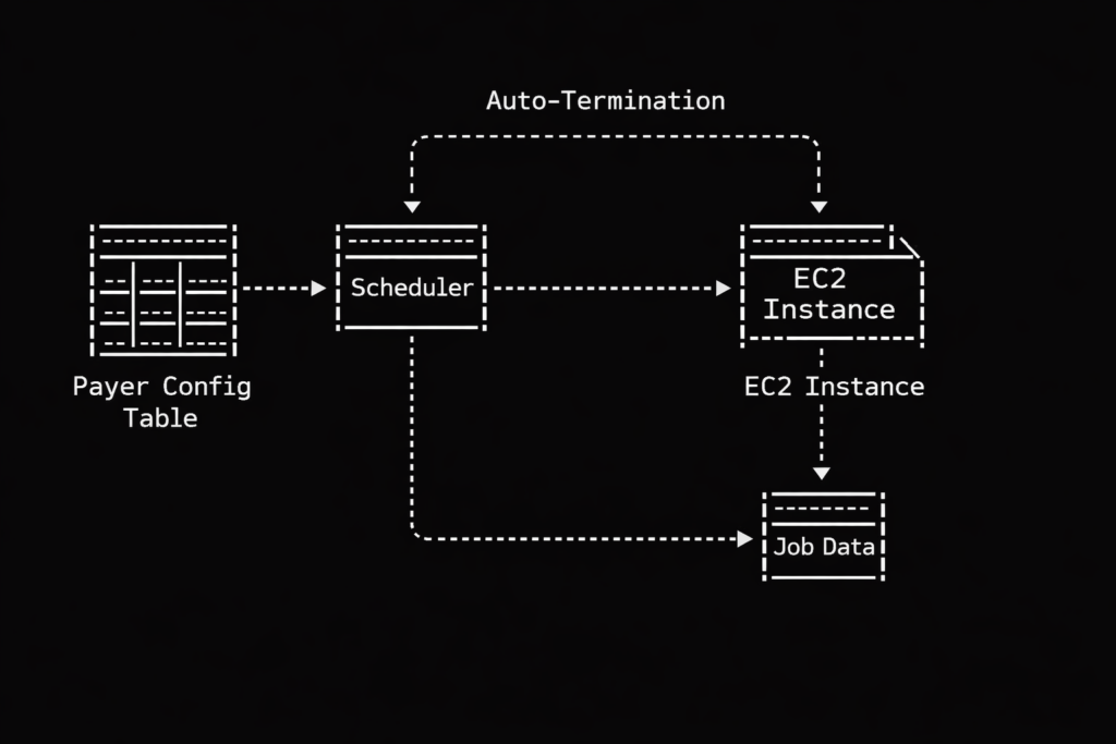
This is why we abandoned the generic approach and built our own dynamic EC2 provisioning system. Instead of maintaining a herd of generic servers waiting around for something to do, we create bespoke servers on demand based on a central configuration table.
The ruthless nightclub bouncer of job scheduling
Let us look at how this actually works regarding prioritization. Our system relies on that central configuration table to dictate order. Think of this table as the guest list at an obnoxiously exclusive nightclub. Our scheduler acts as the ruthless bouncer.
When jobs arrive at the queue, the bouncer checks the list. Member data? Right this way to the VIP lounge, sir. Claims data? Stand on the curb behind the velvet rope until the members are comfortably seated. Generic auto scaling has no native concept of this social hierarchy. It just sees a mob outside the club and opens the front doors wide. Our dynamic approach gives us perfect, tyrannical control over who gets processed first, ensuring our pipelines execute in a beautifully deterministic way. We spin up exactly the compute we specify, exactly when we want it.
Leaving your car running in the garage
Then there is the financial absurdity of warm pools. Standard auto scaling often relies on keeping a baseline of idle instances warm and ready, just in case a payer decides to drop a massive batch of files at two in the morning.
Keeping idle servers running is the technological equivalent of leaving your car engine idling in the closed garage all night just in case you get a sudden craving for a carton of milk at dawn. It is expensive, it is wasteful, and it makes you look a bit foolish when the AWS bill arrives.
Our dynamic system operates with a baseline of zero. We experience one hundred percent burst efficiency because we only pay for the exact compute we use, precisely when we use it. Cost savings happen naturally when you refuse to pay for things that are sitting around doing nothing.
A delightfully brutal server lifecycle
The operational model we ended up with is almost comically simple compared to traditional methods. A generic scaling group requires complex scaling policies, tricky cooldown periods, and endless tweaking of CloudWatch alarms. It is like managing a highly sensitive, moody teenager.
Our dynamic EC2 model is wonderfully ruthless. We create the instance and inject it with a single, highly specific purpose via a startup script. The instance wakes up, processes the healthcare data with absolute precision, and then politely self destructs so it stops billing us. They are the mayflies of the cloud computing world. They live just long enough to do their job, and then they vanish. There are no orphaned instances wandering the cloud.
This dynamic provisioning model has fundamentally altered how we digest payer workloads. We have somehow achieved a weird but perfect holy grail of cloud architecture. We get the granular flexibility of serverless functions, the raw, unadulterated horsepower of dedicated EC2 instances, and the stingy cost efficiency of a pure event-driven design.
If your processing jobs vary wildly from payer to payer, and if you care deeply about enforcing priorities without burning money on idle metal, building a disposable compute army might be exactly what your architecture is missing. We said goodbye to our idle servers, and honestly, we do not miss them at all.
I was at my desk the other day attempting to achieve what passes for serenity in modern IT, which is to say I was watching a Kubernetes cluster behave like a supermarket trolley with one cursed wheel. Everything looked stable in the dashboard, which, in cloud terms, is the equivalent of a toddler saying “I am being very quiet” from the other room.
That was when a younger colleague appeared at the edge of my monitor like a pop-up window you simply cannot close.
“Can I ask you something?” he said.
This phrase is rarely followed by useful inquiries, such as “Where do you keep the biscuits?” It is invariably followed by something philosophical, the kind of question that makes you suddenly aware you have become the person other people treat as a human FAQ.
“Is it worth it?” he asked. “All of this. The studying. The certifications. The on-call shifts. With AI coming to take it all away.”
He did not actually use the phrase “robot overlords”, but it hung in the air anyway, right beside that other permanent office presence, the existential dread that arrives every Monday morning and sits down without introducing itself.
Being “senior” in the technology sector is a funny thing. It is not like being a wise mountain sage who understands the mysteries of the wind. It is more like being the only person in the room who remembers what the internet looked like before it became a shopping mall with a comment section. You are not necessarily smarter. You are simply older, and you have survived enough migrations to know that the universe is largely held together by duct tape and misunderstood configuration files.
So I looked at him, panicked slightly, and decided to tell him the truth.
The accidental trap of the perfect puzzle piece
The problem with the way we build careers, especially in engineering, is that we treat ourselves like replacement parts for a very specific machine. We spend years filing down our edges, polishing our corners, and making sure we fit perfectly into a slot labelled “Java Developer” or “Cloud Architect.”
This strategy works wonderfully right up until the moment the machine decides to change its shape.
When that happens, being a perfect puzzle piece is actually a liability. You are left holding a very specific shape in a world that has suddenly decided it prefers round holes. This brings us to the trap of the specialist. The specialist is safe, comfortable, and efficient. But the specialist is also the first thing to be replaced when the algorithm learns how to do the job faster.
The alternative sounds exhausting. It is the path of the “Generalist.”
To a logical brain that enjoys defined parameters, a generalist looks suspiciously like someone who cannot make up their mind. But in the coming years, the generalist (confusing as they may be) is the only one safe from extinction. The generalist does not ask “Where do I fit?” The generalist asks, “What am I trying to build?” and then learns whatever is necessary to build it. It is less like being a factory worker and more like being a frantic homeowner trying to fix a leak with a roll of tape and a YouTube video. It is messy, but unlike the factory worker, the homeowner cannot be automated out of existence because the problems they solve are never exactly the same twice.
The four horsemen of the career apocalypse
Once you accept that the future will not reward narrow excellence, you stumble upon an equally alarming discovery regarding the skills that actually matter. The usual list tends to circle around four eternal pillars known to induce hives in most engineers: marketing, sales, writing, and speaking.
If you work in DevOps or cloud, these words likely land with the gentle comfort of a cold spoon sliding down your back. We tend to view marketing and sales as the parts of the economy where people smile too much and perhaps use too much hair gel. Writing and public speaking, meanwhile, are often just painful reminders of that time we accidentally said “utilize” in a meeting when “use” would have sufficed.
But here is a useful reframing I have been trying to adopt.
Marketing and sales are not trickery. They are simply “the message“. They are the ability to explain to another human being why something matters. If you have ever tried to convince a Product Manager that technical debt is real and dangerous, you have done sales. If you failed, it was likely because your marketing was poor.
Writing and speaking are not performance art. They are “the medium“. In a world where AI can generate code in seconds, the ability to write clean code becomes less valuable than the ability to write a clean explanation of why we need that code. The modern career is increasingly about communicating value rather than just quietly creating it in a dark room. The “Artist” focuses on the craft. The “Sellout” focuses on the money. The goal, irritating as it may be, is to become the “Artist-Entrepreneur” who respects the craft enough to sell it properly.
The museum of ideas and the art of dissatisfaction
So how does one actually prepare for this vaguely threatening future?
The advice usually involves creating a “Vision Board” with pictures of yachts and people laughing at salads. I have always found this difficult, mostly because my vision usually extends no further than wanting my printer to work on the first try.
A far more effective tool is the “Anti-vision“.
This involves looking at the life you absolutely do not want and running in the opposite direction. It is a powerful motivator. I can quite easily visualize a future of endless Zoom meetings where we discuss the synergy of leverage, and that vision propels me to learn new skills faster than any promise of a Ferrari ever could.
This leads to the concept of curating a “Museum of Ideas”. You do not need to be a genius inventor. You just need to be a curator. You collect the ideas, people, and concepts that resonate with you, and you try to figure out why they work. It is reverse engineering, which is something we are actually good at. We do it with software all the time. Doing it with our careers feels strange, but the logic holds. You look at the result you want, and you work backward to find the source code.
This process requires you to embrace a certain amount of boredom and dissatisfaction. We usually treat boredom as a bug in the system, something to be patched immediately with scrolling or distraction. But boredom is actually a feature. It is the signal that it is time to evolve. AI does not get bored. It will happily generate generic emails until the heat death of the universe. Only a human gets bored enough to invent something better.
The currency of confidence
So, back to the colleague at my desk, who was still looking at me with the expectant face of a spaniel waiting for a treat.
I told him that yes, it is worth it. But the game has changed.
We are moving from an economy of “knowing things” (which computers do better) to an economy of “connecting things” (which is still a uniquely human mess). The future belongs to the people who can see the whole system, not just the individual lines of code.
When the output of AI becomes abundant and cheap, the value shifts to confidence. Not the loud, arrogant confidence of a television pundit, but the quiet confidence of someone who understands the trade-offs. Employers and clients will not pay you for the code; they will pay you for the assurance that this specific code is the right solution for their specific, messy reality. They pay for taste. They pay for trust.
If the robots are indeed coming for our jobs, the safest position is not to stand guard over one tiny task. It is to become the person who can see the entire ridiculous machine, spot the real problem, and explain it in plain English while everyone else is still arguing about which dashboard is lying.
That, happily, remains a very human talent.
Now, if you will excuse me, I have to start building my museum of ideas right after I figure out why my Linux kernel has decided to panic-dump in the middle of an otherwise peaceful afternoon. I suspect it, too, has been reading about the future and just wanted to feel something.
Someone in a zip-up hoodie has just told you that monoliths are architectural heresy. They insist that proper companies, the grown-up ones with rooftop terraces and kombucha taps in the breakroom, build systems the way squirrels store acorns. They describe hundreds of tiny, frantic caches scattered across the forest floor, each with its own API, its own database, and its own emotional baggage.
You stand there nodding along while holding your warm beer, feeling vaguely inadequate. You hide the shameful secret that your application compiles in less time than it takes to brew a coffee. You do not mention that your code lives in a repository that does not require a map and a compass to navigate. Your system runs on something scandalously simple. It is a monolith.
Welcome to the cult of small things. We have been expecting you, and we have prepared a very complicated seat for you.
The insecurity of the monolithic developer
The microservices revolution did not begin with logic. It began with envy. It started with a handful of very successful case studies that functioned less like technical blueprints and more like impossible beauty standards for teenagers.
Netflix streams billions of hours of video. Amazon ships everything from electric toothbrushes to tactical uranium (probably) to your door in two days. Their systems are vast, distributed, and miraculous. So the industry did what any rational group of humans would do. We copied their homework without checking if we were taking the same class.
We looked at Amazon’s architecture and decided that our internal employee timesheet application needed the same level of distributed complexity as a global logistics network. This is like buying a Formula 1 pit crew to help you parallel park a Honda Civic. It is technically impressive, sure. But it is also a cry for help.
Suddenly, admitting you maintained a monolith became a confession. Teams began introducing themselves at conferences by stating their number of microservices, the way bodybuilders flex biceps, or suburban dads compare lawn mower horsepower. “We are at 150 microservices,” someone would say, and the crowd would murmur approval. Nobody thought to ask if those services did anything useful. Nobody questioned whether the team spent more time debugging network calls than writing features.
The promise was flexibility. The reality became a different kind of rigidity. We traded the “spaghetti code” of the monolith for something far worse. We built a distributed bowl of spaghetti where the meatballs are hosted on different continents, and the sauce requires a security token to touch the pasta.
Debugging a murder mystery where the body keeps moving
Here is what the brochures and the medium articles do not mention. Debugging a monolith is straightforward. You follow the stack trace like a detective following footprints in the snow.
Debugging a distributed system, however, is less like solving a murder mystery and more like investigating a haunting. The evidence vanishes. The logs are in different time zones. Requests pass through so many services that by the time you find the culprit, you have forgotten the crime.
Everything works perfectly in isolation. This is the great lie of the unit test. Your service A works fine. Your service B works fine. But when you put them together, you get a Rube Goldberg machine that occasionally processes invoices but mostly generates heat and confusion.
To solve this, we invented “observability,” which is a fancy word for hiring a digital private investigator to stalk your own code. You need a service discovery tool. Then, a distributed tracing library. Then a circuit breaker, a bulkhead, a sidecar proxy, a configuration server, and a small shrine to the gods of eventual consistency.
Your developer productivity begins a gentle, heartbreaking decline. A simple feature, such as adding a “middle name” field to a user profile, now requires coordinating three teams, two API version bumps, and a change management ticket that will be reviewed next Thursday. The context switching alone shaves IQ points off your day. You have solved the complexity of the monolith by creating fifty mini monoliths, each with its own deployment pipeline and its own lonely maintainer who has started talking to the linter.
Your infrastructure bill is now a novelty item
There is a financial aspect to this midlife crisis. In the old days, you rented a server. Maybe two. You paid a fixed amount, and the server did the work.
In the microservices era, you are not just paying for the work. You are paying for the coordination of the work. You are paying for the network traffic between the services. You are paying for the serialization and deserialization of data that never leaves your data center. You are paying for the CPU cycles required to run the orchestration tools that manage the containers that hold the services that do the work.
It is an administrative tax. It is like hiring a construction crew where one guy hammers the nail, and twelve other guys stand around with clipboards coordinating the hammering angle, the hammer velocity, and the nail impact assessment strategy.
Amazon Prime Video found this out the hard way. In a move that shocked the industry, they published a case study detailing how they moved from a distributed, serverless architecture back to a monolithic structure for one of their core monitoring services.
The results were not subtle. They reduced their infrastructure costs by 90 percent. That is not a rounding error. That is enough money to buy a private island. Or at least a very nice yacht. They realized that sending video frames back and forth between serverless functions was the digital equivalent of mailing a singular sock to yourself one at a time. It was inefficient, expensive, and silly.
The myth of infinite scalability
Let us talk about that word. Scalability. It gets whispered in architectural reviews like a magic spell. “But will it scale?” someone asks, and suddenly you are drawing boxes and arrows on a whiteboard, each box a little fiefdom with its own database and existential dread.
Here is a secret that might get you kicked out of the hipster coffee shop. Most systems never see the traffic that justifies this complexity. Your boutique e-commerce site for artisanal cat toys does not need to handle Black Friday traffic every Tuesday. It could likely run on a well-provisioned server and a prayer. Using microservices for these workloads is like renting an aircraft hangar to store a bicycle.
Scalability comes in many flavors. You can scale a monolith horizontally behind a load balancer. You can scale specific heavy functions without splitting your entire domain model into atomic particles. Docker and containers gave us consistent deployment environments without requiring a service mesh so complex that it needs its own PhD program to operate.
The infinite scalability argument assumes you will be the next Google. Statistically, you will not. And even if you are, you can refactor later. It is much easier to slice up a monolith than it is to glue together a shattered vase.
Making peace with the boring choice
So what is the alternative? Must we return to the bad old days of unmaintainable codeballs?
No. The alternative is the modular monolith. This sounds like an oxymoron, but it functions like a dream. It is the architectural equivalent of a sensible sedan. It is not flashy. It will not make people jealous at traffic lights. But it starts every morning, it carries all your groceries, and it does not require a specialized mechanic flown in from Italy to change the oil.
You separate concerns inside the same codebase. You make your boundaries clear. You enforce modularity with code structure rather than network latency. When a module truly needs to scale differently, or a team truly needs autonomy, you extract it. You do this not because a conference speaker told you to, but because your profiler and your sprint retrospectives are screaming it.
Your architecture should match your team size. Three engineers do not need a service per person. They need a codebase they can understand without opening seventeen browser tabs. There is no shame in this. The shame is in building a distributed system so brittle that every deploy feels like defusing a bomb in an action movie, but without the cool soundtrack.
Epilogue
Architectural patterns are like diet fads. They come in waves, each promising total transformation. One decade, it is all about small meals, the next it is intermittent fasting, the next it is eating only raw meat like a caveman.
The truth is boring and unmarketable. Balance works. Microservices have their place. They are essential for organizations with thousands of developers who need to work in parallel without stepping on each other’s toes. They are great for systems that genuinely have distinct, isolated scaling needs.
For everything else, simplicity remains the ultimate sophistication. It is also the ultimate sanity preserver.
Next time someone tells you monoliths are dead, ask them how many incident response meetings they attended this week. The answer might be all the architecture review you need.
(Footnote: If they answer “zero,” they are either lying, or their pager duty alerts are currently stuck in a dead letter queue somewhere between Service A and Service B.)
You press a finger against the greasy glass of your smartphone. You are in a café in Melbourne, the coffee is lukewarm, and you have made the executive decision to watch a video of a cat falling off a Roomba. It feels like a trivial action.
But for the data packet birthed by that tap, this is D-Day.
It is a tiny, nervous backpacker being kicked out into the digital wilderness with nothing but a destination address and a crippling fear of latency. Its journey through Amazon’s cloud infrastructure is not the clean, sterile diagram your systems architect drew on a whiteboard. It is a micro drama of hope, bureaucratic routing, and existential dread that plays out in roughly 200 milliseconds.
We tend to think of the internet as a series of tubes, but it is more accurate to think of it as a series of highly opinionated bouncers and overworked bureaucrats. To understand how your cat video loads, we have to follow this anxious packet through the gauntlet of Amazon Web Services (AWS).
The initial panic and the mapmaker with a god complex
Our packet leaves your phone and hits the cellular network. It is screaming for directions. It needs to find the server hosting the video, but it only has a name (e.g., cats.example.com). Computers do not speak English; they speak IP addresses.
Enter Route 53.
Amazon calls Route 53 a Domain Name System (DNS) service. In practice, it acts like a travel agent with a philosophy degree and multiple personality disorder. It does not just look up addresses; it judges you based on where you are standing and how healthy the destination looks.
If Route 53 is configured with Geolocation Routing, it acts like a local snob. It looks at our packet’s passport, sees “Melbourne,” and sneers. “You are not going to the Oregon server. The Americans are asleep, and the latency would be dreadful. You are going to Sydney.”
However, Route 53 is also a hypochondriac. Through Health Checks, it constantly pokes the servers to see if they are alive. It is the digital equivalent of texting a friend, “Are you awake?” every ten seconds. If the Sydney server fails to respond three times in a row, Route 53 assumes the worst, death, fire, or a kernel panic, and instantly reroutes our packet to Singapore. This is Failover Routing, the prepared pessimist of the group.
The packet doesn’t care about the logic. It just wants an address so it can stop hyperventilating in the void.
CloudFront is the desperate golden retriever of the internet
Armed with an IP address, our packet rushes toward the destination. But hopefully, it never actually reaches the main server. That would be inefficient. Instead, it runs into CloudFront.
CloudFront is a Content Delivery Network (CDN). Think of it as a network of convenience stores scattered all over the globe, so you don’t have to drive to the factory to buy milk. Or, more accurately, think of CloudFront as a Golden Retriever that wants to please you so badly it is vibrating.
Its job is caching. It memorizes content. When our packet arrives at the CloudFront “Edge Location” in Melbourne, the service frantically checks its pockets. “Do I have the cat video? I think I have the cat video. I fetched it for that guy in the corner five minutes ago!”
If it has the video (a Cache Hit), it hands it over immediately. The packet is relieved. The journey is over. Everyone goes home happy.
But if CloudFront cannot find the video (a Cache Miss), the mood turns sour. The Golden Retriever looks guilty. It now has to turn around and run all the way to the origin server to fetch the data fresh. This is the “Edge” of the network, a place that sounds like a U2 guitarist but is actually just a rack of humming metal in a secure facility near the airport.
The tragedy of CloudFront is the Time To Live (TTL). This is the expiration date on the data. If the TTL is set to 24 hours, CloudFront will proudly hand you a version of the website from yesterday, oblivious to the fact that you updated the spelling errors this morning. It is like a dog bringing you a dead bird it found last week, convinced it is still a great gift.
The security guard who judges your shoes
If our packet suffers a Cache Miss, it must travel deeper into the data center. But first, it has to get past the Web Application Firewall (WAF).
The WAF is not a firewall in the traditional sense; it is a nightclub bouncer who has had a very long shift and hates everyone. It stands at the velvet rope, scrutinizing every packet for signs of “malicious intent.”
It checks for SQL injection, which is the digital equivalent of trying to sneak a knife into the club tape-draped to your ankle. It checks for Cross-Site Scripting (XSS), which is essentially trying to trick the club into changing its name to “Free Drinks for Everyone.”
The WAF operates on a set of rules that range from reasonable to paranoid. Sometimes, it blocks a legitimate packet just because it looks suspicious, perhaps the packet is too large, or it came from a country the WAF has decided to distrust today. The packet pleads its innocence, but the WAF is a piece of software code; it does not negotiate. It simply returns a 403 Forbidden error, which translates roughly to: “Your shoes are ugly. Get out.”
The Application Load Balancer manages the VIP list
Having survived the bouncer, our weary packet arrives at the Application Load Balancer (ALB). If the WAF is the bouncer, the ALB is the Maitre D’ holding the clipboard.
The ALB is obsessed with fairness and health. It stands in front of a pool of identical servers (the Target Group) and decides who has to do the work. It is trying to prevent any single server from having a nervous breakdown due to overcrowding.
“Server A is busy processing a login request,” the ALB mutters. “Server B is currently restarting because it had a panic attack. You,” it points to our packet, “you go to Server C. It looks bored.”
The ALB’s relationship with the servers is codependent and toxic. It performs health checks on them relentlessly. It demands a 200 OK status code every thirty seconds. If a server takes too long to reply or replies with an error, the ALB declares it “Unhealthy” and stops sending it friends. It effectively ghosts the server until it gets its act together.
The Origin, where the magic (and heat) happens
Finally, the packet reaches the destination. The Origin.
We like to imagine the cloud as an ethereal, fluffy place. In reality, the Origin is likely an EC2 instance, a virtual slice of a computer sitting in a windowless room in Northern Virginia or Dublin. The room is deafeningly loud with the sound of cooling fans and smells of ozone and hot plastic.
Here, the application code actually runs. The request is processed, and the server realizes it needs the actual video file. It reaches out to Amazon S3 (Simple Storage Service), which is essentially a bottomless digital bucket where the internet hoards its data.
The EC2 instance grabs the video from the bucket, processes it, and prepares to send it back.
This is the most fragile part of the journey. If the code has a bug, the server might vomit a 500 Internal Server Error. This is the server saying, “I tried, but I broke something inside myself.” If the database is overwhelmed, the request might time out.
When this happens, the failure cascades back up the chain. The ALB shrugs and tells the user “502 Bad Gateway” (translation: ” The guy in the back room isn’t talking to me”). The WAF doesn’t care. CloudFront caches the error page, so now everyone sees the error for the next hour.
And somewhere, a DevOps engineer’s phone starts buzzing at 3:00 AM.
The return trip
But today, the system works. The Origin retrieves the video bytes. It hands them to the ALB, which passes them to the WAF (who checks them one last time for contraband), which hands them to CloudFront, which hands them to the cellular network.
The packet returns to your phone. The screen flickers. The cat falls off the Roomba. You chuckle, swipe up, and request the next video.
You have no idea that you just forced a tiny, digital backpacker to navigate a global bureaucracy, evade a paranoid security guard, and wake up a server in a different hemisphere, all in less time than it takes you to blink. It is a modern marvel held together by fiber optics and anxiety.
So spare a thought for the data. It has seen things you wouldn’t believe.