DataEngineering

Keyword search is the friend who hears every word and misses the point. Vector search is the friend who nods, squints a little, and says, “You want a safe family SUV that will not make your wallet cry.” This story is about teaching BigQuery to be the second friend.

I wanted semantic search without renting another database, shipping nightly exports, or maintaining yet another dashboard only I remember to feed. The goal was simple and a little cheeky: keep the data in BigQuery, add embeddings with Vertex AI, create a vector index, and still use boring old SQL to filter by price and mileage. Results should read like good advice, not a word-count contest.

Below is a practical pattern that works well for catalogs, internal knowledge bases, and “please find me the thing I mean” situations. It is light on ceremony, honest about trade‑offs, and opinionated where it needs to be.

Why keyword search keeps missing the point

• Humans ask for meanings, not tokens. “Family SUV that does not guzzle” is intent, not keywords.
  
• Catalogs are messy. Price, mileage, features, and descriptions live in different columns and dialects.
  
• Traditional search treats text like a bag of Scrabble tiles. Embeddings turn it into geometry where similar meanings sit near each other.
  

If you have ever typed “cheap laptop with decent battery” and received a gaming brick with neon lighting, you know the problem.

Keep data where it already lives

No new database. BigQuery already stores your rows, talks SQL, and now speaks vectors. The plan

1. Build a clean content string per row so the model has a story to understand.
   
2. Generate embeddings in BigQuery via a remote Vertex AI model.
   
3. Store those vectors in a table and, when it makes sense, add a vector index.
   
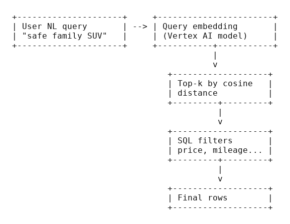
4. Search with a natural‑language query embedding and filter with plain SQL.
   

Map of the idea:

Prepare a clean narrative for each row

Your model will eat whatever you feed it. Feed it something tidy. The goal is a single content field with labeled parts, so the embedding has clues.

-- Demo names and values are fictitious
CREATE OR REPLACE TABLE demo_cars.search_base AS
SELECT
  listing_id,
  make,
  model,
  year,
  price_usd,
  mileage_km,
  body_type,
  fuel,
  features,
  CONCAT(
    'make=', make, ' | ',
    'model=', model, ' | ',
    'year=', CAST(year AS STRING), ' | ',
    'price_usd=', CAST(price_usd AS STRING), ' | ',
    'mileage_km=', CAST(mileage_km AS STRING), ' | ',
    'body=', body_type, ' | ',
    'fuel=', fuel, ' | ',
    'features=', ARRAY_TO_STRING(features, ', ')
  ) AS content
FROM demo_cars.listings
WHERE status = 'active';

Housekeeping that pays off

• Normalize units and spellings early. “20k km” is cute; 20000 is useful.
  
• Keep labels short and consistent. Your future self will thank you.
  
• Avoid stuffing everything. Noise in, noise out.
  

Turn text into vectors without hand waving

We will assume you have a BigQuery remote model that points to your Vertex AI text‑embedding endpoint. Choose a modern embedding model and be explicit about task type, use RETRIEVAL_DOCUMENT for rows and RETRIEVAL_QUERY for user queries. That hint matters.

Embed the documents

-- Store document embeddings alongside your base table
CREATE OR REPLACE TABLE demo_cars.search_with_vec AS
SELECT
  b.listing_id,
  b.make, b.model, b.year, b.price_usd, b.mileage_km, b.body_type, b.fuel, b.features,
  e.ml_generate_embedding_result AS embedding
FROM demo_cars.search_base AS b,
UNNEST([
  STRUCT(
    (SELECT ml_generate_embedding_result
     FROM ML.GENERATE_EMBEDDING(
       MODEL `demo.embed_text`,
       (SELECT b.content AS content),
       STRUCT(TRUE AS flatten_json_output, 'RETRIEVAL_DOCUMENT' AS task_type)
     )) AS ml_generate_embedding_result
  )
]) AS e;

That cross join with a single STRUCT is a neat way to add one vector per row without creating a separate subquery table. If you prefer, materialize embeddings in a separate table and JOIN on listing_id to minimize churn.

Build an index when it helps and skip it when it does not

BigQuery can scan vectors without an index, which is fine for small tables and prototypes. For larger tables, add an IVF index with cosine distance.

-- Optional but recommended beyond a few thousand rows
CREATE VECTOR INDEX demo_cars.search_with_vec_idx
ON demo_cars.search_with_vec(embedding)
OPTIONS(
  distance_type = 'COSINE',
  index_type = 'IVF',
  ivf_options = '{"num_lists": 128}'
);

Rules of thumb

• Start without an index for quick experiments. Add the index when latency or cost asks for it.
  
• Tune num_lists only after measuring. Guessing is cardio for your CPU.
  

Ask in plain English, filter in plain SQL

Here is the heart of it. One short block that embeds the query, runs vector search, then applies filters your finance team actually understands.

-- Natural language wish
DECLARE user_query STRING DEFAULT 'family SUV with lane assist under 18000 USD';

WITH q AS (
  SELECT ml_generate_embedding_result AS qvec
  FROM ML.GENERATE_EMBEDDING(
    MODEL `demo.embed_text`,
    (SELECT user_query AS content),
    STRUCT(TRUE AS flatten_json_output, 'RETRIEVAL_QUERY' AS task_type)
  )
)
SELECT s.listing_id, s.make, s.model, s.year, s.price_usd, s.mileage_km, s.body_type
FROM VECTOR_SEARCH(
  TABLE demo_cars.search_with_vec, 'embedding',
  TABLE q, query_column_to_search => 'qvec',
  top_k => 20, distance_type => 'COSINE'
) AS s
WHERE s.price_usd <= 18000
  AND s.body_type = 'SUV'
ORDER BY s.price_usd ASC;

This is the “hybrid search” pattern, shoulder to shoulder, semantics finds plausible candidates, SQL draws the hard lines. You get relevance and guardrails.

Measure quality and cost without a research grant

You do not need a PhD rubric, just a habit.

Relevance sanity check

• Write five real queries from your users. Note how many good hits appear in the top ten. If it is fewer than six, look at your content field. It is almost always the content.

Latency

• Time the query with and without the vector index. Keep an eye on top‑k and filters. If you filter out 90% of candidates, you can often keep top‑k low.

Cost

• Avoid regenerating embeddings. Upserts should only touch changed rows. Schedule small nightly or hourly batches, not heroic full refreshes.

Where things wobble and how to steady them

Vague user queries

• Add example phrasing in your product UI. Even two placeholders nudge users into better intent.

Sparse or noisy text

• Enrich your content with compact labels and the two or three features people actually ask for. Resist the urge to dump raw logs.

Synonyms of the trade

• Lightweight mapping helps. If your users say “lane keeping” and your data says “lane assist,” consider normalizing in content.

Region mismatches

• Keep your dataset, remote connection, and model in compatible regions. Latency enjoys proximity. Downtime enjoys misconfigurations.

Run it day after day without drama

A few operational notes that keep the lights on

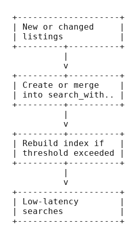
• Track changes by listing_id and only re‑embed those rows.
  
• Rebuild or refresh the index on a schedule that fits your churn. Weekly is plenty for most catalogs.
  
• Keep one “golden query set” around for spot checks after schema or model changes.
  

Takeaways you can tape to your monitor

• Keep data in BigQuery and add meaning with embeddings.
  
• Build one tidy content per row. Labels beat prose.
  
• Use RETRIEVAL_DOCUMENT for rows and RETRIEVAL_QUERY for the user’s text.
  
• Start without an index; add IVF with cosine when volume demands it.
  
• Let vectors shortlist and let SQL make the final call.
  

Tiny bits you might want later

An alternative query that biases toward newer listings

DECLARE user_query STRING DEFAULT 'compact hybrid with good safety under 15000 USD';
WITH q AS (
  SELECT ml_generate_embedding_result AS qvec
  FROM ML.GENERATE_EMBEDDING(
    MODEL `demo.embed_text`,
    (SELECT user_query AS content),
    STRUCT(TRUE AS flatten_json_output, 'RETRIEVAL_QUERY' AS task_type)
  )
)
SELECT s.listing_id, s.make, s.model, s.year, s.price_usd
FROM VECTOR_SEARCH(
  TABLE demo_cars.search_with_vec, 'embedding',
  TABLE q, query_column_to_search => 'qvec',
  top_k => 15, distance_type => 'COSINE'
) AS s
WHERE s.price_usd <= 15000
ORDER BY s.year DESC, s.price_usd ASC
LIMIT 10;

Quick checklist before you ship

• The remote model exists and is reachable from BigQuery.
  
• Dataset and connection share a region you actually meant to use.
  
• content strings are consistent and free of junk units.
  
• Embeddings updated only for changed rows.
  
• Vector index present on tables that need it and not on those that do not.
  

If keyword search is literal‑minded, this setup is the polite interpreter who knows what you meant, forgives your typos, and still respects the house rules. You keep your data in one place, you use one language to query it, and you get answers that feel like common sense rather than a thesaurus attack. That is the job.